Spatial Interpolation Using Ordinary Kriging • climateBR

Introduction

Spatial interpolation is commonly used to estimate meteorological variables at locations where no direct observations are available. The kriging_inmet() function implements ordinary kriging using weather station observations and spatial prediction locations provided as sf objects.

This vignette demonstrates how to interpolate accumulated rainfall from INMET weather stations.

library(climateBR)
library(dplyr)
library(sf)
library(ggplot2)
library(patchwork)

Input Data

The example uses rainfall observations from the 2024 Rio Grande do Sul flood event together with municipality geometries.

data("floods_rs")
data("mun_stations")

# Alternative to: geobr::read_municipality(year = 2024)
tmp <- tempfile(fileext = ".rda")
on.exit(unlink(tmp), add = TRUE)

download.file(
  "https://github.com/kaiorb52/dados_municipais/raw/main/mun_24.rda",
  destfile = tmp,
  mode = "wb"
)

load(tmp)

The station observations are converted to an sf object and projected to a planar coordinate reference system, which is required for distance-based spatial analysis.

rain_sf <- floods_rs |>
  st_as_sf(coords = c("lon", "lat"), crs = 4326) |>
  st_transform(crs = 29193)

mun_centroid <- mun_24 |>
  select(code_muni, geom) |>
  mutate(
    ponto = st_point_on_surface(geom)
  ) |>
  st_drop_geometry()

mun_grid_sf <- mun_centroid |>
  st_as_sf() |>
  st_transform(crs = 29193)

Running the Kriging Model

The kriging_inmet() function computes an empirical variogram, fits a spherical variogram model, and performs ordinary kriging predictions for the target locations.

krig_result <- kriging_inmet(
  stations_df = rain_sf,
  mun_geo     = mun_grid_sf
)
#> [using ordinary kriging]

The predicted values (var1.pred) and prediction variances (var1.var) are then attached to the municipality dataset.

mun_pred <- mun_centroid |>
  select(code_muni) |>
  bind_cols(
    krig_result |>
      st_drop_geometry() |>
      select(
        precip_krig     = var1.pred,
        precip_krig_var = var1.var
      )
  )

Visualizing Kriging Predictions

The following map displays municipality-level rainfall estimates obtained through ordinary kriging.

p1 <- mun_24 |>
  left_join(mun_pred, by = "code_muni") |>
  ggplot() +
  geom_sf(aes(fill = precip_krig), color = NA) +
  labs(title = "Ordinary Kriging") +
  scale_fill_distiller(
    palette = "RdYlGn",
    direction = 1,
    na.value = "grey80"
  ) +
  theme_void() +
  theme(
    legend.position = c(0.9, 0.1)
  )

Comparison with the Nearest-Station Approach

For comparison, the map below assigns each municipality the rainfall value from its closest weather station.


data("inmet_stations")

mun_stations2 <- mun_stations |> 
  left_join(inmet_stations |> select(code_wmo, creation_year)) |> 
  filter(creation_year <= 2024) |> 
  arrange(distance) |> 
  distinct(code_ibge7, .keep_all = TRUE)

mun_floods <- floods_rs |>
  left_join(
    mun_stations2,
    by = c("code_wmo" = "code_wmo")
  )

p2 <- mun_24 |>
  left_join(
    mun_floods |>
      select(code_ibge7, total_rainfall),
    by = c("code_muni" = "code_ibge7")
  ) |>
  ggplot() +
  geom_sf(aes(fill = total_rainfall), color = NA) +
  labs(title = "Nearest Station") +
  scale_fill_distiller(
    palette = "RdYlGn",
    direction = 1,
    na.value = "grey80"
  ) +
  theme_void() +
  theme(
    legend.position = c(0.9, 0.1)
  )

The figure below compares rainfall estimates generated using ordinary kriging against values obtained from the nearest-station approach.

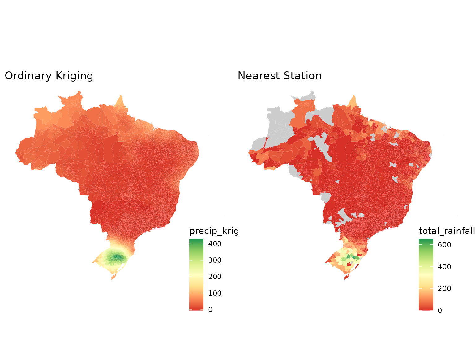
Ordinary kriging generally produces smoother spatial surfaces and incorporates information from multiple nearby stations, whereas the nearest-station method assigns the same value to all municipalities linked to a given station and may introduce abrupt spatial discontinuities.

Each approach has advantages and limitations:

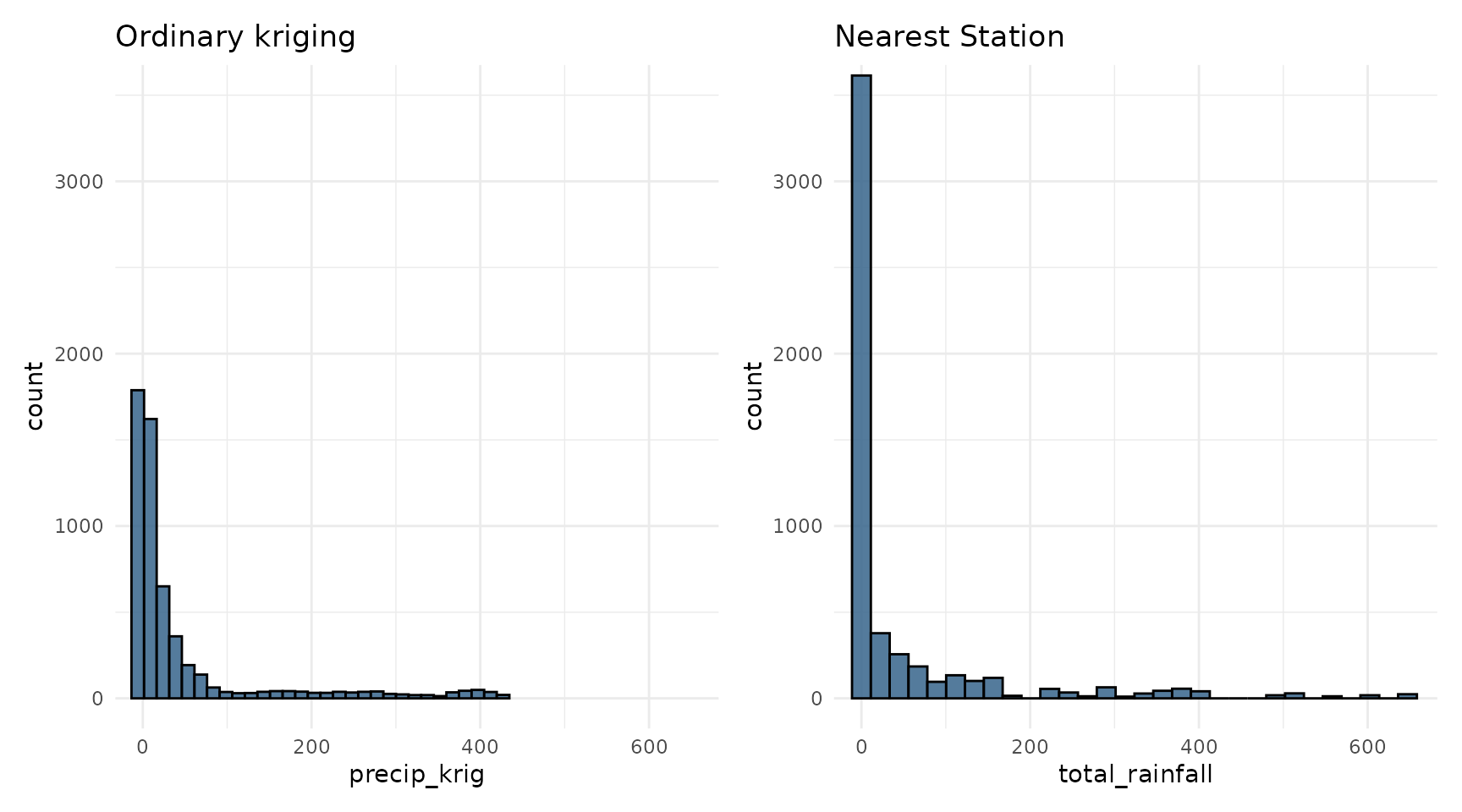
Ordinary kriging accounts for spatial dependence and usually produces more realistic spatial patterns. However, as a statistical interpolation method, it can produce physically impossible values (such as negative rainfall) and tends to smooth the surface, so very high rainfall totals may be underestimated.
Nearest station preserves the observed values, including extremes. However, many municipalities may share the same station, which creates large areas with identical values and artificial boundaries between neighboring municipalities. Real rainfall does not change abruptly at these boundaries.

The histograms below compare the distribution of municipality-level estimates from both approaches.